Correlation vs. Causation: Simpson’s Paradox Example
Two things changing together may reflect a causal effect, reverse influence, a shared driver or sampling choices. The hard work is deciding which explanation the study design can support.
Compare rates before inferring an explanation
The Simpson Paradox and Group Rate Checker is an original browser tool that adds successes and totals across two named categories. It reports the category-specific rates and the combined rates and flags a clear sign reversal. The numbers default to a hypothetical comparison of two homework strategies across easy and hard tasks. Because the worksheet uses actual counts rather than precomputed percentages, the aggregation can be independently verified. It does not assume anyone was randomized or provide a causal estimate.
For paired continuous observations, Lynara already has a different tool, the Pearson Correlation Calculator. Pearson's r describes a linear association; it does not turn a relationship into an experiment. The stratified-rate worksheet answers a different question about mixing categories and changes in group composition. Both belong in a research student's checking process, but they are not interchangeable methods.
Association means a pattern, not a mechanism
Suppose a classroom dataset shows students who spend longer on practice questions tend to receive higher test scores. This is an association worth investigating. It does not, by itself, show that adding 30 minutes of practice will increase a particular student's result. Previous subject knowledge, class attendance, tutoring, age, motivation or different test versions may influence both practice time and score. Students with higher marks might also enjoy practicing more, reversing the implied direction of influence.
Observational data can be valuable even when it cannot establish causation. An honest conclusion might be, “In this sample, reported practice duration was positively associated with quiz score.” The conclusion should name the sample, time period, variables and known limitations. “Practice caused a 20% increase” requires stronger evidence: a defined outcome and intervention, an appropriate comparison, consideration of the causal alternatives and an analysis matching the design. A correlation coefficient cannot provide those missing design elements.
What a confounder actually does
A confounder is not simply any extra variable in a spreadsheet. In a causal question, it can create or distort the association because it relates to the variable of interest and the outcome in ways the data-generating process makes relevant. For example, in a fictional homework comparison, task difficulty affects the chance of success. If students choose one strategy more frequently for easy tasks and another for hard tasks, a pooled score comparison mixes strategy choice with the distribution of difficulty. The comparison can look very different after separating easy and hard tasks.
The Penn State regression methods lesson examines omitted predictors and shows how the direction of a fitted relationship can change after relevant variables are included. This is a warning to inspect the mechanism and design rather than always trust the first coefficient. But “control for everything” is not a safe rule either: conditioning on a variable affected by the treatment, or a common consequence of other variables, can introduce a different form of bias. Identify the causal question first.
Worked classroom example: both categories favor B, but the total favors A
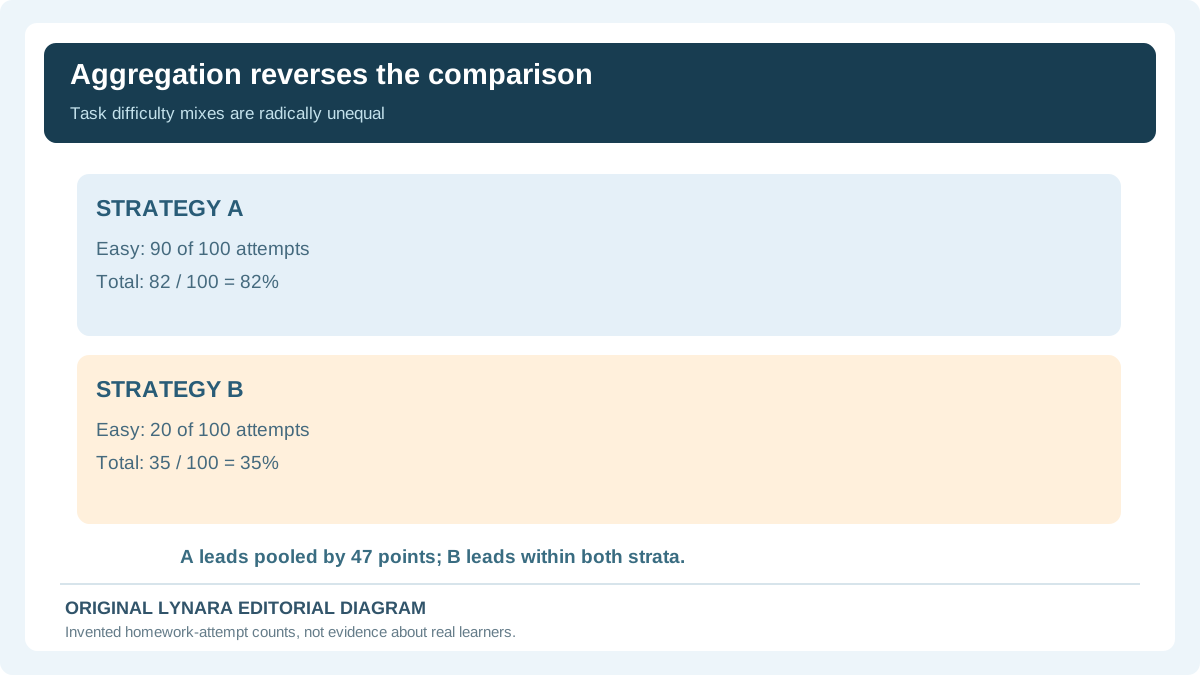
Consider two fictional homework approaches labeled A and B, each used for some easy and hard exercises. The records below are made up for arithmetic teaching; they are not evidence that a real learning strategy works. For easy tasks, A has 81 correct answers in 90 attempts, or 90%, while B has 19 in 20, or 95%. For hard tasks, A has 1 correct answer in 10 attempts, or 10%, while B has 16 in 80, or 20%. In both categories, B has the better recorded rate: five percentage points higher on easy tasks, ten points higher on hard tasks.
Now add the counts rather than average the two percentages equally. Strategy A has 81 + 1 = 82 successes out of 100, or 82%. Strategy B has 19 + 16 = 35 successes out of 100, or 35%. The pooled result therefore favors A by 47 percentage points even though both category comparisons favor B. There is no arithmetic error: 90 of A's 100 attempts were easy, while only 20 of B's were easy. The two approaches were observed under very different mixes of task difficulty.
Enter these counts in the stratified rate checker. It will show category-level B minus A differences of +5 and +10 percentage points and a pooled B minus A difference of −47 percentage points. Those signs form a Simpson-style reversal. The numbers are deliberately easy to audit; a “paradox” here means the conclusion depends on how groups are combined, not that 82 and 35 are impossible or that the higher within-category strategy is automatically the correct causal choice.

Why different group weights can reverse a result
A combined success rate is a weighted average of the success rates inside its groups. For A, 90% of attempts are in the easy category, so the aggregate is 0.90 × 90% + 0.10 × 10% = 82%. For B, only 20% are easy, so the aggregate is 0.20 × 95% + 0.80 × 20% = 35%. The rate in each category and the proportion of observations in that category both affect the final total. This is why merely averaging 90% and 10% to get 50% would be incorrect for A's actual count mix.
The Stanford Encyclopedia of Philosophy entry on Simpson's paradox explores how aggregate and subgroup relationships can disagree and why causality requires additional reasoning. A classroom comparison does not automatically reveal whether the correct estimand is the actual aggregate performance, a standardized equal-mix comparison or something else. That depends on whether the question asks what happened in the observed workload or what would happen if the strategies faced comparable tasks.
A reversal is not proof of discrimination or a treatment effect
The historical university-admissions example often used to teach Simpson's paradox highlights how applicant distributions across departments can affect aggregate admission rates. The key methodological issue is not whether the data can be made to “say anything”; it is which question each rate answers. Department composition may matter, and a causal analysis must account for selection into departments and other relevant processes. Do not transfer a stylized reversal directly to claims about an actual institution, population or individual.
An University of Illinois Chicago explanation offers a separate worked illustration showing why unstratified comparisons can mislead. The peer-reviewed practical guide by Kievit and colleagues discusses the phenomenon in psychological research. Neither reference implies that simply grouping by the variable with the largest effect always produces a valid causal conclusion. One must understand which variables existed before an intervention and which may themselves be consequences of other factors.
How confounding differs from reverse causation
Imagine that a school observes a positive relationship between stress and time spent studying. Stress may prompt students to study longer, or studying under deadline pressure may increase stress, or a third factor such as exam difficulty may influence both. Without the collection timeline and a research design, a single correlation cannot separate these possibilities. “Reverse causation” asks whether the proposed effect may actually influence the supposed cause. Confounding asks whether another factor can explain some of the measured association. Both can operate together.
Useful practical questions include: Which variable was measured first? Could participants choose their own activity? Is the sample limited to students who completed the assessment? Did the data exclude absent students? Is there a variable such as prior achievement that influenced both? Does the study report how those factors were measured or modeled? These are questions for methods sections and data provenance, not instructions to automatically remove a variable because a coefficient looks inconvenient.
Nonlinearity and outliers make single-number summaries fragile
Even a correctly computed Pearson correlation measures a specific kind of linear association. A curved relationship can have a weak linear correlation while still showing a strong, systematic pattern. A small number of extreme observations can drive a fitted line or obscure patterns among the bulk of records. Plot the actual paired measurements when permitted, label units and consider whether the relationship differs across relevant categories. A positive coefficient is not a universal “strength of influence” score.
For any actual paired dataset, calculate Pearson's r only when the data shape and assumptions suit the assignment; then read the scatterplot and think about plausible selection and measurement errors. Our Pearson Correlation Calculator is linked here for transparent computation, but cannot discover unmeasured confounders or reconstruct randomization from raw numbers. The separate Chart Axis and Denominator Checker can help inspect misleading graph scales, yet its two-point arithmetic does not establish a population-wide relationship.
Observational comparisons versus intervention designs
Researchers may collect survey answers or routine class scores without controlling who uses which study technique. That is an observational comparison. Researchers may instead randomly assign eligible participants to clearly defined conditions, measure outcomes consistently and report how missing data were handled. Random assignment can help reduce preexisting differences in expectation, but it is not magic: noncompliance, attrition, measurement bias, chance and failures of study conduct still matter. The strength of a causal conclusion depends on what was done and measured, not merely on whether the word “experiment” appears in the abstract.
For a classroom project, define the claim in terms the design can actually support. If students chose their own study strategy, a descriptive comparison of their recorded outcomes may be defensible; a claim that one method necessarily raises grades would be unwarranted. If the work includes interviews, surveys and scores, review our qualitative versus quantitative research guide to distinguish research questions and measurement approaches before selecting a statistical method.
Check denominators, missingness and repeated students
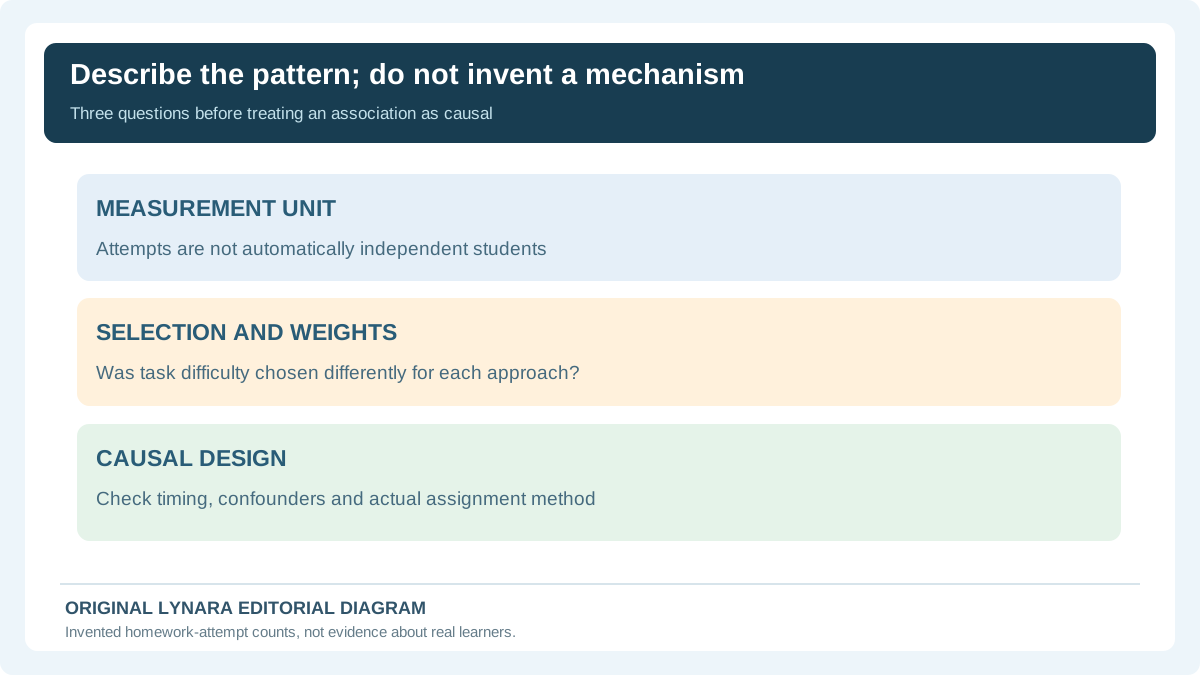
Group-level rates must refer to a clear denominator. “A had 81 successes” is incomplete if we do not know whether the group attempted 90 or 500 tasks. Repeated attempts from one participant may not be independent observations. The fictional worksheet counts attempts, not unique students, because the example never claims the latter. If a real student takes several easy tasks and another takes one hard task, treating every attempt as an independent student may bias uncertainty estimates. The tool therefore performs descriptive arithmetic only, without p-values or confidence intervals.
Make a data dictionary specifying the success definition, difficulty classification, each observation's unit and the handling of missing tasks. If a category is missing entirely for one strategy, the checker refuses a zero denominator instead of inventing a 0% success rate. For small authorized data exports, our Research CSV Quality Checker can help identify structural problems in pasted CSV; it does not validate that labels or responses are correct. Preserve raw source records and document any changes, as explained in our reproducible spreadsheet guide.
When pooling might answer a valid question
It is tempting to conclude that subgroup results are always superior because they look more detailed. That is too simplistic. If your question is “Which strategy produced more correct answers for its actual collection of assignments this term?” the observed pooled rates describe those recorded workloads. If your question is “Which strategy would perform better for a comparable mix of tasks?” the pooled rates mix unequal assignments and do not answer the hypothetical equal-mix question on their own. Both calculations may be numerically correct while addressing different estimands.
Statistical models, standardization and experimental designs may help answer more targeted questions, but each comes with assumptions. You cannot turn the difference in two weighted means into a fair comparison by declaring it so, and changing strata after looking at the result risks cherry-picking. Document why the categories were chosen and which comparison was planned. The worksheet's job is to make category weights visible; it does not decide whether a particular adjustment is scientifically justified.
A defensible paragraph for a student assignment
For the made-up example, a student could write: “Across the recorded attempts, approach A had an 82% completion rate and B had a 35% rate. However, A was used for easy tasks in 90% of its attempts, compared with 20% for B. Within easy tasks the rate was 90% for A and 95% for B; within hard tasks it was 10% for A and 20% for B. The direction of the overall comparison therefore reverses when task difficulty is considered. These descriptive counts do not establish that either approach caused higher performance.” This makes the numbers and the limitation visible rather than hiding the apparent contradiction.
When using actual research, replace every figure and category name with the verified study's data and cite the original methods. Do not present a synthetic teaching example as observed evidence. An AI assistant can help brainstorm explanations for a relationship, but it may overstate what the data prove. Ask it to list alternatives and assumptions, then verify those suggestions against the paper's methods and the relevant literature.
Final research checklist
Identify the intended causal claim, the population and the unit of observation. Check how participants were selected, whether they could choose exposure, what came first in time and which variables could influence both the exposure and outcome. Compute all necessary denominators. Inspect category-specific and pooled rates, and ask whether the category composition differs. Do not automatically treat an impressive reversal as evidence that the higher subgroup rate is a causal benefit. When the purpose is numerical correlation rather than grouped completion rates, switch to the appropriate calculator instead of forcing your data into two successes-and-totals tables.
Start with the Simpson Paradox and Group Rate Checker and edit the four supplied cells to see how weighting changes results. Continue to the research graph reading guide to learn how scales and labels can affect the visual presentation of these same facts. A strong student report should leave the reader able to reproduce the numbers and distinguish a defensible association from a causal conclusion that the study cannot support.
A reproducible subgroup-versus-pooled rate audit
Copy the four invented source cells into a worksheet instead of asking an AI model to summarize two headline percentages. In easy tasks, approach A has 81 successes from 90 attempts and B has 19 from 20. In hard tasks, A has 1 from 10 and B has 16 from 80. Subgroup rates therefore favor B: 95% versus 90% for easy tasks and 20% versus 10% for hard. When outcomes are pooled, A has 82/100 = 82% correct and B has 35/100 = 35% correct. Neither calculation contradicts the other; the two groups faced different task mixes.
| Difficulty | Approach A | Approach B | Who leads? |
|---|---|---|---|
| Easy | 81 / 90 = 90% | 19 / 20 = 95% | B by 5 points |
| Hard | 1 / 10 = 10% | 16 / 80 = 20% | B by 10 points |
| Pooled | 82 / 100 = 82% | 35 / 100 = 35% | A by 47 points |
Now inspect the weights. Ninety percent of A's attempts are easy, while only twenty percent of B's are easy. This imbalance can explain the reversal without inventing an arithmetic error or a special psychological effect. The Stanford Encyclopedia of Philosophy explains that the direction of an association can change after combining data strata and that causal reasoning must determine which comparison addresses the question.
The classroom worksheet counts attempts, not independent students. If one student completes twenty easy problems and another attempts a single difficult one, a naive statistical model that treats every attempt as a new independent learner can give misleading uncertainty estimates. Because this example provides no random assignment, sample-design information, confidence intervals or preexisting knowledge measures, the article reports only transparent arithmetic and not an effect of one method on grades.
An alternative question might ask how the approaches would compare under the same difficulty distribution. You would have to choose that target workload and apply an appropriate weighting or design. Simply dividing by the observed total answers does not estimate a common-difficulty causal effect. Similarly, equal-weight averaging the two subgroup percentages without stating that a fifty-fifty difficulty mix is the target answers a hypothetical question rather than reproducing the observed totals.
Use the Stratified Rate Reversal Checker to reproduce the source counts, and document what was counted. If a later source includes duplicated observations or unknown task difficulty, stop and resolve that data-quality issue before drawing an inference. In the final paragraph, identify the population, the unit of measurement and what the comparison can and cannot show.