How to Read Research Graphs: Axes, Rates and Uncertainty
A convincing chart may still be easy to misread. Learn to check who was measured, what the axes mean and whether the claim matches the actual numbers.
Try the paired chart-reading checker
Our Research Chart Axis and Denominator Checker compares two values, a visible axis minimum, and—where relevant—each group's numerator and denominator. It calculates true differences, relative changes and the different bar lengths a truncated baseline can produce. It does not read chart images automatically, validate statistical sampling or claim that a named paper deliberately misled readers. This guide teaches the questions a student must ask before using that output in a report.
Read the figure caption before the shape
In a research article, the image and figure caption work as a pair. Start with the population studied, collection period, measurement definition and source notes. A line rising from left to right looks convincing, but it could depict mean scores from four participants, a national survey with confidence intervals or a hypothetical model with assumptions. Those situations support different conclusions. Read the caption and methods before saying the data represent all students, all countries or a causal effect.
For every figure, write a one-sentence description that does not overclaim: “Among the observed records in this sample, the reported mean increased between two measured dates.” Then ask whether the study explains missing measurements, the time interval and uncertainty. An article may contain multiple panels showing raw counts, model estimates and standardized results. Do not combine them because their curves look similar. A transparent research summary identifies the specific figure panel and the number or estimate used.
Axis names, units and scale come before the trend
Look at the horizontal and vertical axes. One may show months or participant groups; the other may show dollars, temperature, test points or a rate per 100,000 people. Units are essential: 20 people, 20% and 20 incidents per 100,000 are not interchangeable. Determine whether the vertical scale is linear or logarithmic and whether a percentage has a natural 0–100 range. A chart's plotted value can be meaningful while its design leads the eye to an exaggerated conclusion.
The UK Office for National Statistics guidance on axes and gridlines explains why labels and scale choices deserve attention and warns about confusing dual-axis displays. Its official design service discusses charts as a way to communicate comparisons, not a replacement for supplying definitions and context. Rather than automatically calling a chart deceptive because its axis is unusual, note exactly how the scale changes the visual reading.
Why bar-chart baselines matter more than most students expect
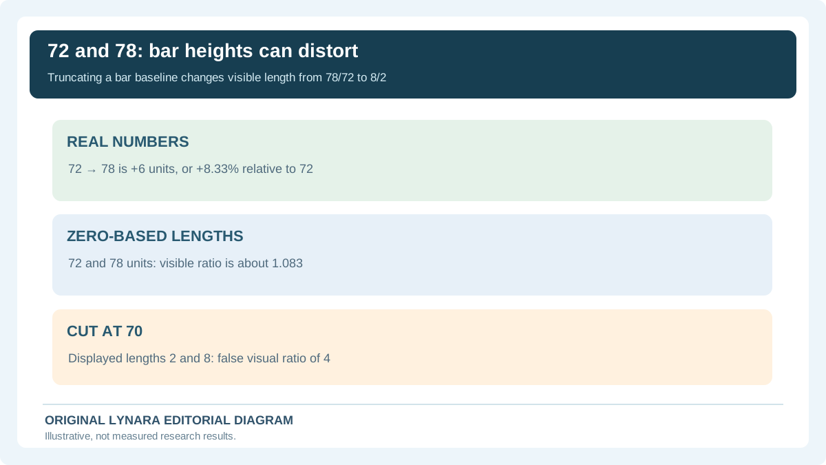
A bar chart typically represents a quantity by the length of each rectangular bar. Imagine a fictional classroom report with scores of 72 and 78 units. If the vertical bars start at zero, their heights are 72 and 78. The second bar is 78 ÷ 72 ≈ 1.083 times the first in numerical magnitude. But if the designer truncates the baseline to 70, the displayed heights become 2 and 8 units. Those visible lengths now have a ratio of 4 to 1, even though the underlying values did not change.
The arithmetic tells us the second value is six units higher, a relative increase of 6 ÷ 72 × 100 = 8.33%. It does not justify the statement “four times as high.” This example is intentionally invented so the computation can be independently checked. The ONS discussion of bar-chart baselines explains the special risk of changing a bar's apparent length through the displayed axis start. The axis checker reproduces this 72-versus-78 example and shows both ratios.
Line charts are different: a nonzero axis is not always dishonest
A line graph usually encodes the position of points and how a variable changes across an ordered sequence. A narrow y-axis range can be informative when researchers study small but meaningful fluctuations. The important question becomes whether the axis is labeled, the range makes the context understandable and the time intervals are genuinely comparable. A rule claiming that every line chart must begin at zero would hide useful information in some circumstances.
The ONS article about line-chart axes specifically distinguishes the positional encoding of lines from the length encoding of bars. It does not suggest all truncated scales are ideal: the choice should serve the task and be clear to the reader. If the horizontal positions correspond to unequal time periods, check whether the plotted spacing reflects the actual intervals. Drawing an evenly spaced line from 2019 to 2020 and then to 2026 may conceal a five-year gap when treated as equal steps.
One chart can mix counts, percentages and rates
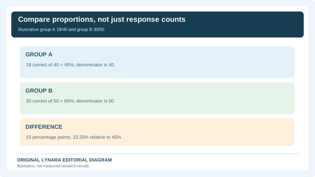
Suppose a fictional report compares correct responses in two student groups. In group A, 18 of 40 answered correctly. In group B, 30 of 50 did. A raw-count graph shows 18 and 30; because the groups have different sizes, a fair comparison of the proportion answering correctly needs the denominator. Group A's rate is 18 ÷ 40 × 100 = 45%, and group B's is 30 ÷ 50 × 100 = 60%. A claim that B was “12 better” is meaningless unless you say the units are students. For percentage results, group B is 15 percentage points higher.
Its relative increase is (60 − 45) ÷ 45 × 100 = 33.33%. That is not the same as a 33.33-percentage-point increase. The denominator matters especially when comparing different years, subgroups or populations. A country with more recorded incidents may have a lower rate per resident when its population is much larger. The matching chart checker has a rates mode so students can calculate group-specific percentages from actual numerator and denominator inputs instead of relying on visually similar bars.
Read uncertainty intervals before ranking two estimates
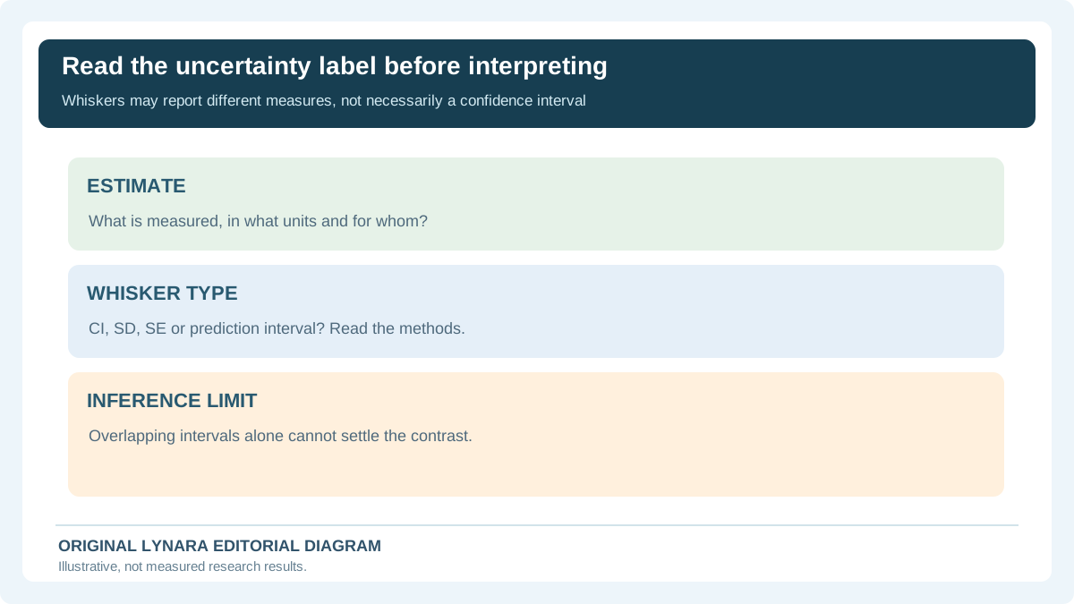
Many research papers plot estimates with whiskers, shading or ribbons. Those may represent confidence intervals, credible intervals, standard deviations, standard errors, data ranges or prediction intervals. The meanings are not interchangeable. The caption and methods should tell you which measure was used, at what level, and how it was constructed. A narrow interval is not automatically proof of a large real-world effect or a good research design. An estimate's reliability also depends on sampling, measurement and study assumptions.
If two reported averages are close, do not declare one group universally better based solely on the taller bar. Nor should you assume overlapping confidence intervals always imply no statistically significant difference: the appropriate comparison depends on the particular estimated contrast and methodology. When a question requires hypothesis testing, see our separate statistical test selection guide and study-design checker. Neither one certifies that a plotted interval in a third-party paper was calculated correctly.
Logarithmic scales deserve a deliberate rereading
On a linear scale, equally spaced ticks represent equal numerical differences. On a logarithmic scale, equally spaced ticks represent equal multiplicative changes, such as 1, 10, 100 and 1,000. This can be useful when values span orders of magnitude, but the reader must recognize the transformation. A visual step between 10 and 100 is an increase of 90, while the step between 100 and 1,000 is an increase of 900, although both represent a tenfold multiplication. Treat a constant slope on a log plot differently from a constant slope on a standard linear plot.
Log scales are not simply “fake statistics”; they help reveal proportional changes that a linear scale would conceal. They are inappropriate or require extra explanation for some zero or negative-value situations. Look for axis labels, tick spacing, whether the figure says logarithmic, and whether the paper's conclusions use raw or transformed values. Our baseline checker is deliberately limited to comparing two points on a conventional numeric value scale; it is not a log-axis reconstruction tool.
Watch for missing categories and unequal comparison windows
Research visualizations often omit categories to keep a figure readable. Sometimes they group small categories into “Other,” exclude missing data or show only observations with complete records. Those choices can affect the displayed pattern. Find the sample sizes in the caption or methods. A bar representing 5 of 6 observed responses should not be described as representing an entire class of 30 without acknowledging the missing records. When the missing cases are systematic, the distortion may be larger than the data-quality checker can detect from a formatted chart.
In a time series, the window matters too. A graph showing one week before a policy change and two years afterward should not be summarized as a balanced before-and-after experiment. Seasonal patterns, selection criteria and measurement changes could matter. The Statistics Canada guide to line charts illustrates how axis scales and intervals alter the apparent pattern. Always use the underlying reported measurement periods when writing the takeaway.
Correlation in a figure is not a causal explanation
A scatterplot may show that observations with more practice time tend to have higher quiz scores. That can be a genuine association without proving the extra practice caused the score difference. Prior ability, attendance, motivation, tutoring or different test versions could affect both. A regression line summarizes a model under assumptions; it is not by itself a controlled experiment. The direction of the relationship may be ambiguous, and a small number of outliers can strongly affect the trend.
For a reliable classroom write-up, name the variables and population, state whether the result is descriptive or inferential, and report the association without overstating causal meaning. If the paper claims causation, examine the study design and controls. Our existing Pearson Correlation Calculator answers a separate mathematical question for paired numerical observations; it does not establish whether the original paper's data were collected independently or ethically.
Keep raw data quality separate from the presentation quality
Even a beautifully labeled chart may be built from duplicated records, inconsistent units or missing participant responses that the article does not disclose. Conversely, clean data can be presented poorly. If researchers provide a supplementary CSV, data dictionary or analysis code, use it to understand how observations became the plotted values. Do not silently rewrite the published graph merely because you think a different chart looks better. Compare the original publication, caption and underlying tables, and document any recomputation.
Our Research CSV Quality Checker can identify exact repeated rows, blank cells and structural inconsistencies in a small local file, without uploading the data. The companion spreadsheet reproducibility guide shows how to preserve raw values and document changes. These tools are not evidence that any paper's dataset is authentic. They support practical checks after the data owner has lawfully shared the data and the reader has permission to examine it.
How to describe a graph in an assignment without overstating it
A useful interpretation has three levels. First, describe the observed values and units: “The reported average changed from 72 to 78 points.” Second, calculate the size of the difference: “This is six points, or an 8.33% increase relative to 72.” Third, explain the limits: “The figure alone does not show whether the difference is statistically meaningful or caused by an intervention.” Those statements are precise and do not require pretending you have repeated the research.
Avoid writing that “the graph proves” when the only evidence is the picture's upward slope. Ask whether a plausible alternative explanation exists, whether the estimate is uncertain, and whether the sample is representative of the wider population. An AI assistant may describe the most dramatic visual feature or invent a numerical scale if you provide a blurry screenshot. Transcribe the exact published values, check them against the article's table, and do the arithmetic yourself or with a transparent local tool.
Final checklist before citing a research figure
Record the author, date, paper, figure number and panel. Confirm what one observation represents, how many observations are included, the chart type, axis units, start and end points, any log transformations, missing-value rules and uncertainty definition. Recalculate any difference, percentage-point change or relative percentage described in your text. Identify where the paper draws a causal conclusion and whether its design supports that claim. If an axis choice seems exaggerated, report the numerical values rather than speculating about the author's motive.
For immediate practice, enter the fictional 72-versus-78 example in the Chart Axis and Denominator Checker. Next try 18/40 and 30/50 as separate group rates. Then select an actual figure from an assigned article, verify its source numbers and describe what the chart does—and does not—establish. This is the skill a chart summary should teach: not a prettier paraphrase, but a careful reading that another student could independently reproduce.
Audit a chart in four minutes without inventing data
Start by locating the caption, figure number, study sample and measurement units. Reproduce the actual values from a table or downloadable source before describing an apparent trend. A fictional bar comparison with scores 72 and 78 may look dramatically different if its axis starts at 70: displayed lengths become 2 and 8, producing an apparent four-to-one ratio. Yet the underlying result is only 6 units higher, or 6/72 × 100 = 8.33% relative to the first value. The UK Office for National Statistics axes guidance calls for zero-based bars because bar length represents magnitude. It also notes that line and scatter charts can reasonably use cropped ranges with clear labeling, which is why one rigid axis rule does not fit every visualization.
| Group | Correct | Total | Rate |
|---|---|---|---|
| A | 18 | 40 | 45% |
| B | 30 | 50 | 60% |
Next inspect denominators. Group B has 12 more correct responses in the made-up example, but it also has ten more observations. The appropriate comparison of success proportions is 60% versus 45%, a gap of 15 percentage points or 33.33% relative to A. Neither calculation establishes why group B differed. Check whether the units are unique people or repeated tasks, whether missing responses were excluded and whether the two groups were selected comparably.
Finally ask what the uncertainty marks mean. Error bars could represent a standard deviation, standard error, confidence interval or prediction interval. These quantities make different claims, and overlapping confidence intervals are not a universal decision rule for a difference. Look for the contrast's own analysis and methods. The article's companion Chart Axis and Denominator Checker allows local arithmetic checks, but does not authenticate a research graph or validate a causal interpretation.
Use an evidence-based release decision: GO if the underlying values, denominators, caption meaning and design limitations are traceable; REVISE if a sentence mixes relative percent change with percentage points; HOLD if an unlabeled interval, cropped axis or blurry screenshot prevents reliable reconstruction. Include a figure number and original source reference rather than citing a model's image description as evidence.